
merge method.Intro
In this post, I discuss the relationship between the Pandas merge function (and Pandas merge method), and the Pandas join method, and then show examples of how to merge Pandas dataframes with the merge method. Along the way, I describe two useful merge method parameters: the validate parameter, and the indicator parameter.
This article is the second in our Professional Pandas blog post series. The goal of this series is to teach best practices about writing professional-grade Pandas code. If you have questions or topics that you would like to dive into, please reach out on Twitter to @ponderdata or @__mharrison__, and if you’d like to see the notebook version of this blogpost, you can find it on Github here.
(Note: This content is modified from the author’s book, Effective Pandas.)
Joining Data
Terminology Refresher: Method vs. Function
Pandas often has one, two, three, or even more ways to do something. This paradox of choice can be overwhelming. (Indeed software engineering purists would say “There should be one– and preferably only one –obvious way to do it.”) However, here we are with Pandas joining.
In short, there is :
- The
.joinmethod found on a DataFrame - The
.mergemethod found on a DataFrame - The
pd.mergefunction found in the Pandas namespace (pd) - The
pd.concatfunction to horizontally or vertically stack data - Various methods that align on the index and work similar to some joins (like using
df.assign(**other_df))
A Quick Aside on the Python Language
A Python class defines methods. Methods are called on an instance of a class. In the Pandas world, we often have a DataFrame (df) or Series (s) instance. We could call the merge method by saying:
df.merge(another_df)
However, there is also a function, merge. Generally, when folks use Pandas they import the library like this:
import pandas as pd
Since pd is the module where the Pandas merge function is available, you can call the merge function like this:
pd.merge(df, another_df)
Some think that in this last example that merge is a method on pd. That is not correct. If we change the import to load the function, we could run the code like this:
from pandas import merge

merge(df, another_df)
If you aren’t familiar with the difference between methods and functions and would like to explore more, check out the Python tutorial.
End of the Aside
From this author's point of view, forget that the Pandas merge function and the join method exist. You can get along just fine only using the merge method (which I will often refer to in this article as .merge with a period in front as a reminder that it needs to be called on the instance).
In fact, if you dig into the implementation of .join, you will see that it calls the concat or merge functions. Don't waste your brain power trying to keep them straight. Just ignore the merge function and the join method.
One final note, I wish that .merge was named .join because everyone coming from a database world knows what a join is, but .merge offers a little more functionality, hence my recommendation to favor it.
A Short Overview of Joining
Feel free to skip this if you are familiar with database joins. It shows the basic joins using some sales data. Our task might be to find products with no sales, sales that don’t have products, or only sales for products that we have information for.
The supported join types for .merge (specified with the how parameter) are:
'left'– Keep all values from the merging column DataFrame the method was called on.'right'– Keep all values from the merging column of therightDataFrame the method was called on.'inner'– Keep the intersection of all values from the merging columns.'outer'– Keep the union of all values from the merging columns.'cross'– For every row in the instance dataframe, combine with every row from therightDataFrame.
import pandas as pd
products = pd.DataFrame({'id': [1, 3, 10], 'product':
                         ['Cat food', 'Sparkling Water', 'Apple Fritter']})
sales = pd.DataFrame({'product_id': [1, 3, 1, 1, 15],
                      'cost': [4.99, .99, 4.99, 4.99*.8, 7.45]})
Left Join
>>> # keep all *id* columns
>>> products.merge(sales, left_on='id', right_on='product_id', how='left')
    id  product     product_id  cost
0   1   Cat food    1.0     4.990
1   1   Cat food    1.0     4.990
2   1   Cat food    1.0     3.992
3   3   Sparkling Water 3.0     0.990
4   10  Apple Fritter   NaN     NaN
Right Join
>>> # keep all *product_id* columns
>>> products.merge(sales, left_on='id', right_on='product_id', how='right')
    id  product     product_id  cost
0   1.0 Cat food    1       4.990
1   3.0 Sparkling Water 3       0.990
2   1.0 Cat food    1       4.990
3   1.0 Cat food    1       3.992
4   NaN NaN     15      7.450
Inner Join
>>> products.merge(sales, left_on='id', right_on='product_id', how='inner')
    id  product     product_id  cost
0   1   Cat food    1       4.990
1   1   Cat food    1       4.990
2   1   Cat food    1       3.992
3   3   Sparkling Water 3       0.990
Outer Join
>>> products.merge(sales, left_on='id', right_on='product_id', how='outer')
    id  product     product_id  cost
0   1.0 Cat food    1.0     4.990
1   1.0 Cat food    1.0     4.990
2   1.0 Cat food    1.0     3.992
3   3.0 Sparkling Water 3.0     0.990
4   10.0    Apple Fritter   NaN     NaN
5   NaN NaN     15.0        7.450
Cross Join
A merge you might not be aware of is the cross join. This repeats every row of the dataframe with every row that it is merged with. (So this gets big real fast).
>>> # cross join
>>> products.merge(sales, how='cross')
    id  product     product_id  cost
0   1   Cat food    1       4.990
1   1   Cat food    3       0.990
2   1   Cat food    1       4.990
3   1   Cat food    1       3.992
4   1   Cat food    15      7.450
5   3   Sparkling Water 1       4.990
6   3   Sparkling Water 3       0.990
7   3   Sparkling Water 1       4.990
8   3   Sparkling Water 1       3.992
9   3   Sparkling Water 15      7.450
10  10  Apple Fritter   1       4.990
11  10  Apple Fritter   3       0.990
12  10  Apple Fritter   1       4.990
13  10  Apple Fritter   1       3.992
14  10  Apple Fritter   15      7.450
A cross join might come in hand if you need to create all the permutations of some values. In this example, all ways to select three different values from four or ten.
>>> nums = pd.DataFrame({'values':[4, 10]})
>>> (nums
...  .merge(nums, how='cross')
...  .merge(nums, how='cross')
... )
    values_x    values_y    values
0   4       4       4
1   4       4       10
2   4       10      4
3   4       10      10
4   10      4       4
5   10      4       10
6   10      10      4
7   10      10      10
Validation Using the Pandas Merge Method
I will sometimes use a .pipe method to track the size of my data before and after the merge. If you are doing a lot of merges, this will be a snippet of code you will want to keep around.
(Check out the article Professional Pandas: The Pandas Assign Method for more examples of the .pipe method.)
>>> def debug_shape(a_df, comment=''):
...     print(f'{a_df.shape} {comment}')
...     return a_df

>>> (products
...  .pipe(debug_shape, 'before merge')
...  .merge(sales, left_on='id', right_on='product_id', how='outer')
...  .pipe(debug_shape, 'after merge')
... )
(3, 2) before merge
(6, 4) after merge
    id  product     product_id  cost
0   1.0 Cat food    1.0     4.990
1   1.0 Cat food    1.0     4.990
2   1.0 Cat food    1.0     3.992
3   3.0 Sparkling Water 3.0     0.990
4   10.0    Apple Fritter   NaN     NaN
5   NaN NaN     15.0        7.450
A very nice feature of the Pandas merge method is the validate parameter. It allows us to specify if our merge should be one to one ('1:1'), one to many ('1:m'), many to one ('m:1'), or many to many ('m:m').
If your data grows much faster after a merge that might be because you are merging on duplicate values. In our example, the product_id repeats in the products DataFrame. If we were expecting only a single row for the Cat food product and one row from sales for each row from product, we could pass in validate='1:1' parameter.
In this case, Pandas complains that the entries from sales are not unique. This is because there were multiple sales for the Cat food product:
>>> (products
...  .merge(sales, left_on='id', right_on='product_id', how='outer',
...         validate='1:1')
... )
---------------------------------------------------------------------------
MergeError                                Traceback (most recent call last)
 in
      1 (products
      2  .merge(sales, left_on='id', right_on='product_id', how='outer',
----> 3         validate='1:1')
      4 )

3 frames
/usr/local/lib/python3.7/dist-packages/pandas/core/reshape/merge.py in _validate(self, validate)
   1428             elif not right_unique:
   1429                 raise MergeError(
-> 1430                     "Merge keys are not unique in right dataset; not a one-to-one merge"
   1431                 )
   1432

MergeError: Merge keys are not unique in right dataset; not a one-to-one merge
We would need to use validate='1:m' on this example:
>>> (products
...  .merge(sales, left_on='id', right_on='product_id', how='outer',
...         validate='1:m')
... )
    id  product     product_id  cost
0   1.0 Cat food    1.0     4.990
1   1.0 Cat food    1.0     4.990
2   1.0 Cat food    1.0     3.992
3   3.0 Sparkling Water 3.0     0.990
4   10.0    Apple Fritter   NaN     NaN
5   NaN NaN     15.0        7.450
(Note that specifying validate='m:m' can't ever fail, but it could be a nice indicator to whoever reads the code next.)
One more parameter to be aware of is the indicator parameter. This allows us to create a new column indicating which DataFrame the resulting row came from. In this example we specify that the new column should be named side:
>>> (products
...  .merge(sales, left_on='id', right_on='product_id', how='outer',
...         indicator='side')
... )
    id  product     product_id  cost    side
0   1.0 Cat food    1.0     4.990   both
1   1.0 Cat food    1.0     4.990   both
2   1.0 Cat food    1.0     3.992   both
3   3.0 Sparkling Water 3.0     0.990   both
4   10.0    Apple Fritter   NaN     NaN left_only
5   NaN NaN     15.0        7.450   right_only
Example: Joining Dirty Devil Flow and Weather Data Using the Pandas Merge Method
Now let’s look at a real-world example.
We are going to explore data from the Dirty Devil river. This is a river in Utah that the author had some interest in floating down. However, it is only floatable during a small period of time each year. This analysis was part of his attempt to determine when would be a good time to float down this river.
I have some historic data about the flow of the Dirty Devil river on my Github. Let’s load the flow (cubic feet per second, or cfs) and gage height data. In this case we will leave the datetime column as a column and not use it for the index:
>>> import pandas as pd
>>> url = 'https://github.com/mattharrison/datasets/raw/master'\
...     '/data/dirtydevil.txt'
>>> df = pd.read_csv(url, skiprows=lambda num: num <34 or num == 35,
...                  sep='\t')
>>> def to_denver_time(df_, time_col, tz_col):
...     return (df_
...      .assign(**{tz_col: df_[tz_col].replace('MDT', 'MST7MDT')})
...      .groupby(tz_col)
...      [time_col]
...      .transform(lambda s: pd.to_datetime(s)
...          .dt.tz_localize(s.name, ambiguous=True)
...          .dt.tz_convert('America/Denver'))
...     )

>>> def tweak_river(df_):
...     return (df_
...      .assign(datetime=to_denver_time(df_, 'datetime', 'tz_cd'))
...      .rename(columns={'144166_00060': 'cfs',
...                       '144167_00065': 'gage_height'})
...     )

>>> dd = tweak_river(df)
>>> dd
/usr/local/lib/python3.7/dist-packages/IPython/core/interactiveshell.py:3326: DtypeWarning: Columns (7) have mixed types.Specify dtype option on import or set low_memory=False.
  exec(code_obj, self.user_global_ns, self.user_ns)
    agency_cd   site_no     datetime            tz_cd   cfs 144166_00060_cd gage_height 144167_00065_cd
0   USGS        9333500     2001-05-07 01:00:00-06:00   MDT 71.00   A:[91]      NaN     NaN
1   USGS        9333500     2001-05-07 01:15:00-06:00   MDT 71.00   A:[91]      NaN     NaN
2   USGS        9333500     2001-05-07 01:30:00-06:00   MDT 71.00   A:[91]      NaN     NaN
3   USGS        9333500     2001-05-07 01:45:00-06:00   MDT 70.00   A:[91]      NaN     NaN
4   USGS        9333500     2001-05-07 02:00:00-06:00   MDT 70.00   A:[91]      NaN     NaN
... ...     ...     ...             ... ... ...     ...     ...
539300  USGS        9333500     2020-09-28 08:30:00-06:00   MDT 9.53    P       6.16        P
539301  USGS        9333500     2020-09-28 08:45:00-06:00   MDT 9.20    P       6.15        P
539302  USGS        9333500     2020-09-28 09:00:00-06:00   MDT 9.20    P       6.15        P
539303  USGS        9333500     2020-09-28 09:15:00-06:00   MDT 9.20    P       6.15        P
539304  USGS        9333500     2020-09-28 09:30:00-06:00   MDT 9.20    P       6.15        P
539305 rows × 8 columns
I’m also going to load some meteorological data from Hanksville, Utah, a city nearby the river. We will then use the Pandas merge method to join both datasets together so we have flow data as well as temperature and precipitation information.
Some of the columns that are interesting are:
- DATE – Date
- PRCP – Precipitation in inches
- TMIN – Minimum temperature (F) for day
- TMAX – Maximum temperature (F) for day
- TOBS – Observed temperature (F) when measurement made
>>> url = 'https://github.com/mattharrison/datasets/raw/master/data/'\
...       'hanksville.csv'
>>> temp_df = pd.read_csv(url)
>>> def tweak_temp(df_):
...     return (df_
...            .assign(DATE=pd.to_datetime(df_.DATE)
...                 .dt.tz_localize('America/Denver', ambiguous=False))
...            .loc[:,['DATE', 'PRCP', 'TMIN', 'TMAX', 'TOBS']]
...     )
>>> temp_df = tweak_temp(temp_df)
>>> temp_df
    DATE                PRCP    TMIN    TMAX    TOBS
0   2000-01-01 00:00:00-07:00   0.02    21.0    43.0    28.0
1   2000-01-02 00:00:00-07:00   0.03    24.0    39.0    24.0
2   2000-01-03 00:00:00-07:00   0.00    7.0 39.0    18.0
3   2000-01-04 00:00:00-07:00   0.00    5.0 39.0    25.0
4   2000-01-05 00:00:00-07:00   0.00    10.0    44.0    22.0
... ...             ... ... ... ...
6843    2020-09-20 00:00:00-06:00   0.00    46.0    92.0    83.0
6844    2020-09-21 00:00:00-06:00   0.00    47.0    92.0    84.0
6845    2020-09-22 00:00:00-06:00   0.00    54.0    84.0    77.0
6846    2020-09-23 00:00:00-06:00   0.00    47.0    91.0    87.0
6847    2020-09-24 00:00:00-06:00   0.00    43.0    94.0    88.0
6848 rows × 5 columns
Joining Data
Let's use the Pandas merge method to merge by date. This method will try to merge by columns that have the same name, but our dataframes don't have overlapping column names. The dd dataframe has a datetime column and temp_df has a DATE column. We can use the left_on and right_on parameters to help it know how to align the data. The merge method tries to do an inner join by default. That means that rows with values that are the same in the merge columns will be joined together:
>>> (dd
... .merge(temp_df, left_on='datetime', right_on='DATE')
... )
    agency_cd   site_no     datetime            tz_cd   cfs 144166_00060_cd gage_height 144167_00065_cd DATE                PRCP    TMIN    TMAX    TOBS
0   USGS        9333500     2001-05-08 00:00:00-06:00   MDT 75.00   A:[91]      NaN     NaN     2001-05-08 00:00:00-06:00   0.0 43.0    85.0    58.0
1   USGS        9333500     2001-05-09 00:00:00-06:00   MDT 64.00   A:[91]      NaN     NaN     2001-05-09 00:00:00-06:00   0.0 36.0    92.0    64.0
2   USGS        9333500     2001-05-10 00:00:00-06:00   MDT 54.00   A:[91]      NaN     NaN     2001-05-10 00:00:00-06:00   0.0 50.0    92.0    67.0
3   USGS        9333500     2001-05-11 00:00:00-06:00   MDT 56.00   A:[91]      NaN     NaN     2001-05-11 00:00:00-06:00   0.0 46.0    87.0    60.0
4   USGS        9333500     2001-05-12 00:00:00-06:00   MDT 49.00   A:[91]      NaN     NaN     2001-05-12 00:00:00-06:00   0.0 45.0    93.0    72.0
... ...     ...     ...             ... ... ...     ...     ...     ...             ... ... ... ...
4968    USGS        9333500     2020-09-20 00:00:00-06:00   MDT 6.04    P       6.04        P       2020-09-20 00:00:00-06:00   0.0 46.0    92.0    83.0
4969    USGS        9333500     2020-09-21 00:00:00-06:00   MDT 6.83    P       6.07        P       2020-09-21 00:00:00-06:00   0.0 47.0    92.0    84.0
4970    USGS        9333500     2020-09-22 00:00:00-06:00   MDT 6.83    P       6.07        P       2020-09-22 00:00:00-06:00   0.0 54.0    84.0    77.0
4971    USGS        9333500     2020-09-23 00:00:00-06:00   MDT 7.68    P       6.10        P       2020-09-23 00:00:00-06:00   0.0 47.0    91.0    87.0
4972    USGS        9333500     2020-09-24 00:00:00-06:00   MDT 9.86    P       6.17        P       2020-09-24 00:00:00-06:00   0.0 43.0    94.0    88.0
4973 rows × 13 columns
This appears to have worked, but is somewhat problematic. Remember that the dd dataset has a 15-minute frequency, but temp_df only has daily data, so we are only using the value from midnight. We should probably use our resampling skills to calculate the median flow value for each date and then merge. In that case we will want to use the index of the grouped data to merge, so we specify left_index=True:
>>> (dd
...  .groupby(pd.Grouper(key='datetime', freq='D'))
...  .median()
...  .merge(temp_df, left_index=True, right_on='DATE')
... )
    site_no     cfs     gage_height DATE                PRCP    TMIN    TMAX    TOBS
492 9333500.0   71.50       NaN     2001-05-07 00:00:00-06:00   0.0 41.0    82.0    55.0
493 9333500.0   69.00       NaN     2001-05-08 00:00:00-06:00   0.0 43.0    85.0    58.0
494 9333500.0   63.50       NaN     2001-05-09 00:00:00-06:00   0.0 36.0    92.0    64.0
495 9333500.0   55.00       NaN     2001-05-10 00:00:00-06:00   0.0 50.0    92.0    67.0
496 9333500.0   55.00       NaN     2001-05-11 00:00:00-06:00   0.0 46.0    87.0    60.0
... ...     ...     ...     ...             ... ... ... ...
6843    9333500.0   6.83        6.07        2020-09-20 00:00:00-06:00   0.0 46.0    92.0    83.0
6844    9333500.0   6.83        6.07        2020-09-21 00:00:00-06:00   0.0 47.0    92.0    84.0
6845    9333500.0   7.39        6.09        2020-09-22 00:00:00-06:00   0.0 54.0    84.0    77.0
6846    9333500.0   7.97        6.11        2020-09-23 00:00:00-06:00   0.0 47.0    91.0    87.0
6847    9333500.0   9.53        6.16        2020-09-24 00:00:00-06:00   0.0 43.0    94.0    88.0
6356 rows × 8 columns
That looks better (and gives us a few more rows of data).
Validating Joined Data
Let's validate that we had a one-to-one join, i.e. each date from the flow data matched up with a single date from the temperature data. We can use the validate parameter to do this:
>>> (dd
...  .groupby(pd.Grouper(key='datetime', freq='D'))
...  .median()
...  .merge(temp_df, left_index=True, right_on='DATE', how='inner',
...         validate='1:1')
... )
    site_no     cfs gage_height DATE                PRCP    TMIN    TMAX    TOBS
492 9333500.0   71.50   NaN     2001-05-07 00:00:00-06:00   0.0 41.0    82.0    55.0
493 9333500.0   69.00   NaN     2001-05-08 00:00:00-06:00   0.0 43.0    85.0    58.0
494 9333500.0   63.50   NaN     2001-05-09 00:00:00-06:00   0.0 36.0    92.0    64.0
495 9333500.0   55.00   NaN     2001-05-10 00:00:00-06:00   0.0 50.0    92.0    67.0
496 9333500.0   55.00   NaN     2001-05-11 00:00:00-06:00   0.0 46.0    87.0    60.0
... ...     ... ...     ...             ... ... ... ...
6843    9333500.0   6.83    6.07        2020-09-20 00:00:00-06:00   0.0 46.0    92.0    83.0
6844    9333500.0   6.83    6.07        2020-09-21 00:00:00-06:00   0.0 47.0    92.0    84.0
6845    9333500.0   7.39    6.09        2020-09-22 00:00:00-06:00   0.0 54.0    84.0    77.0
6846    9333500.0   7.97    6.11        2020-09-23 00:00:00-06:00   0.0 47.0    91.0    87.0
6847    9333500.0   9.53    6.16        2020-09-24 00:00:00-06:00   0.0 43.0    94.0    88.0
6356 rows × 8 columns
Because this did not raise a MergeError, we know that our data had non-repeating date fields.
Visualization of Data Joined with the Pandas Merge Method
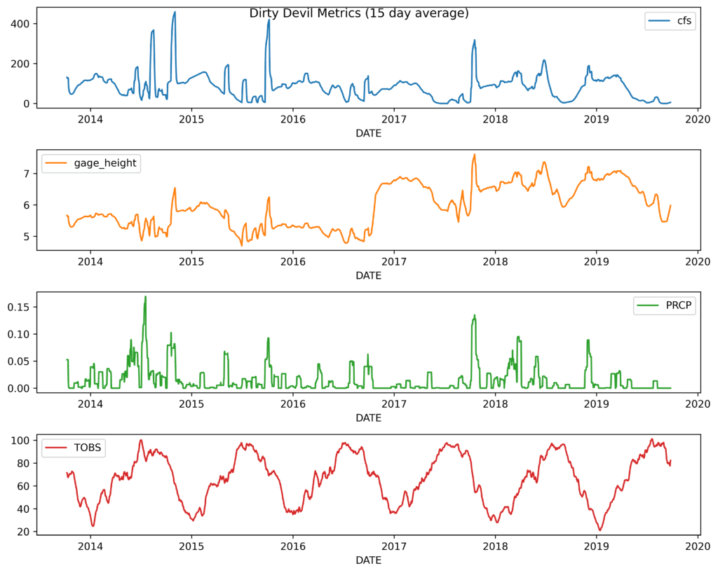
I'm a big fan of visualization. Let's visualize the merged time series. We will add on to our merge chain, stick the date in the index (so that we can plot it on the x-axis), pull out the years from 2014 forward, use the cfs (cubic feet per second), gage_height, PRCP, and TOBS columns, interpolate the missing values, do a rolling 15-day average, and plot the result in their own subplot:
import matplotlib.pyplot as plt
fig, ax = plt.subplots(dpi=600, figsize=(10,8))
(dd
 .groupby(pd.Grouper(key='datetime', freq='D'))
 .median()
 .merge(temp_df, left_index=True, right_on='DATE', how='inner',
        validate='1:1')
 .set_index('DATE')
 .loc['2014':,['cfs', 'gage_height', 'PRCP', 'TOBS']]
 .interpolate()
 .rolling(15)
 .mean()
 .plot(subplots=True, ax=ax)
)
fig.suptitle('Dirty Devil Metrics (15-day average)')
fig.tight_layout()
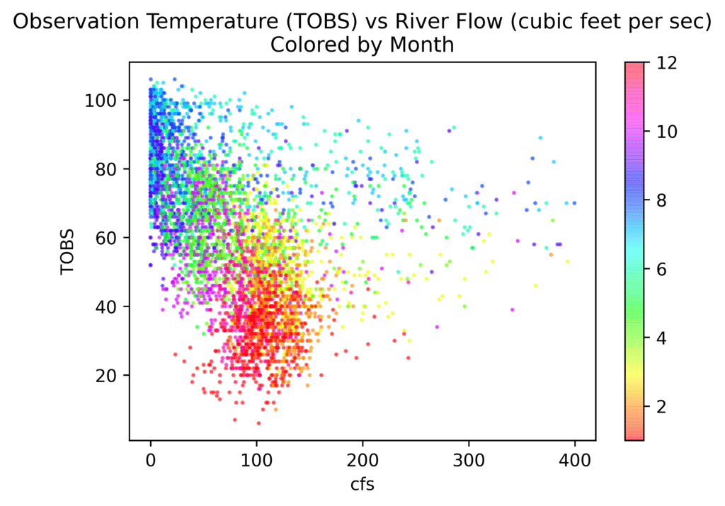
Here’s another plot that is kind of cool once you piece together what is happening. It is a scatterplot of temperature against river flow. I’m coloring this by month of the year. You can see the start of the year at the bottom of the plot. As the year progresses and the temperature warms up, the cfs goes up a little, and then as summer hits, the river almost dries up. During the fall, it starts to cool off and the river starts running higher:
fig, ax = plt.subplots(dpi=600)
dd2 = (dd
 .groupby(pd.Grouper(key='datetime', freq='D'))
 .median()
 .merge(temp_df, left_index=True, right_on='DATE', how='inner',
        validate='1:1')
 .query('cfs < 400')
)
(dd2
 .plot.scatter(x='cfs', y='TOBS', c=dd2.DATE.dt.month,
               ax=ax, cmap='hsv', alpha=.5, s=2)
)
ax.set_title('Observation Temperature (TOBS) '
   'vs River Flow (cubic feet per sec)\nColored by Month')
Summary
Data can often have more utility if we combine it with other data. In the '70s, relational algebra was invented to describe various joins among tabular data. The Pandas merge method of the DataFrame lets us apply these operations to tabular data in the Pandas world. This post explored using the Pandas merge method and the parameters you can use to validate your joining logic.
We would love to hear your feedback. Was this helpful? Did you learn anything new? Tag @ponderdata and @__mharrison__ on Twitter with your insights, and follow both for more content like this. And feel free to suggest new topics you’d like us to dive into for our next Professional Pandas blog post!